Boundary Pruning

These are tools to partition a space into similar regions based on the relative similarity of different areas as well as the complexity of the boundary.

Algorithm

To do so, the space is first filled with all boundaries so that there is a boundary between every pixel of the field. Boundary costs are then calculated based on a number of methods. Then, the highest cost boundary is removed until a threshold number of boundaries is reached. This cutoff is determined by the absolute energy of the last removed boundary or the fraction of boundaries remaining.

Methods of determining cost include:

• Inhomogeneity: cost determined by the change in field values across boundaries.
• Perimeter to Area: take the perimeter / area ratio as the cost, determing fully the polygons formed by all boundaries.
• Both: use both to determine the cost. This requires a constant to weight the two contributions appropriately.

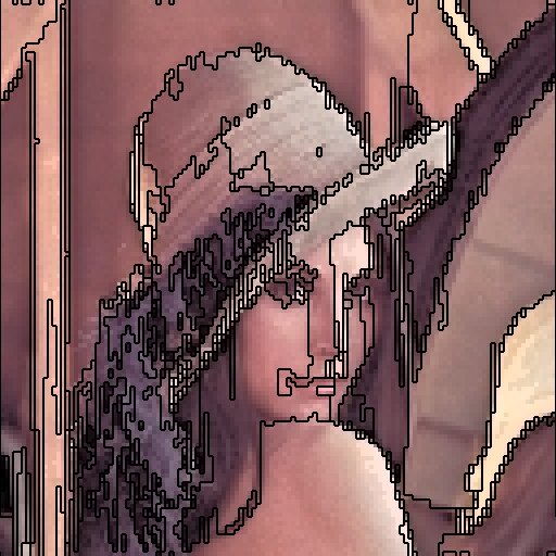
Example

Let’s look at how to use the class. As an example, we will exmploy the stereotypical portrait named ‘Lena’ often used in the graphics industry.

# standard imports
import scipy
from scipy.misc import imread

# the boundary pruning class
import BoundaryPruningMethod as BPM

# open up lena, and set the output prefix
data   = imread("lena.jpg")
output = "output/lena_pruning"

J = 0.1
N = data.shape[0]

# set up the initial boundaries
system = BPM.Initialization(N, data)
boundaries,clusters = system.GenerateClustersFromEverySite()

# perform the actual clustering, this time with both score types
clustering = BPM.ClusteringMixed(N, data, boundaries, clusters, J)
clustering.Run(output)
clustering.GetReconstructionWithBoundary(N, data, output)

The output from this simple example is

Module Listing