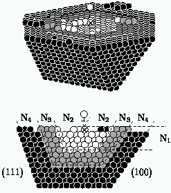
What are these methods, and why did we need to hybridize them? The need comes from the vast differences in time scales...
The collision of an atom with the surface happens very quickly: our Molecular Dynamics simulation (which solves for the motion of the atoms near the collision) ends within five picoseconds (5 x 10-12 seconds, or 1/200,000,000,000 second). The surfaces are grown, however, very slowly: typically one layer of atoms is added each second. If we ran our Molecular Dynamics code until the next collision, we'd wait about a year before the second atom hits!
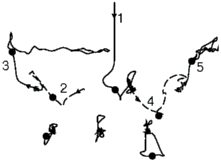
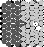
 Here you can see some of the complicated collisions that occur. On the left
you see the trajectory of the atoms as atom number one hits from above. On
the right you can see collisions (side view, then top view) that started
with a straight step edge on the surface, and atom number one hitting from
above, well within the taller region. Notice first that the collisions
leave a mess behind: we quickly lost hope that we could just do each kind
of collision once and keep track of all the answers! Note second that the
net number of atoms on the upper terrace is different for the two
cases. If atom number one gently landed on the upper surface, it would sit
in the third layer (and be colored white). The upper collision pushed the
atom into the second layer: we call it an insertion. The lower
collision bounced atom number three onto the top layer: we call it a
pile-up. Pile-ups and insertions will become important later.
Here you can see some of the complicated collisions that occur. On the left
you see the trajectory of the atoms as atom number one hits from above. On
the right you can see collisions (side view, then top view) that started
with a straight step edge on the surface, and atom number one hitting from
above, well within the taller region. Notice first that the collisions
leave a mess behind: we quickly lost hope that we could just do each kind
of collision once and keep track of all the answers! Note second that the
net number of atoms on the upper terrace is different for the two
cases. If atom number one gently landed on the upper surface, it would sit
in the third layer (and be colored white). The upper collision pushed the
atom into the second layer: we call it an insertion. The lower
collision bounced atom number three onto the top layer: we call it a
pile-up. Pile-ups and insertions will become important later.
 So how do we speed up the calculation in between these tiny, fast collisions?
Between collisions, the atoms mostly wiggle in place. (That's what solids do:
they spend most of their time not flowing around.) Once in a great while,
especially near the surface, an atom will hop from one crystal site to
another.
So how do we speed up the calculation in between these tiny, fast collisions?
Between collisions, the atoms mostly wiggle in place. (That's what solids do:
they spend most of their time not flowing around.) Once in a great while,
especially near the surface, an atom will hop from one crystal site to
another.
Kinetic Monte Carlo saves the computer a huge amount of time by skipping the wiggle-in-place part and just jumping around. We can calculate how often an atom will jump from one site to another, given the arrangement of the nearby atoms. We make big lists of atoms with each arrangment of neighbors, and figure out whose turn it is to hop next.
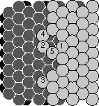
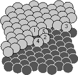
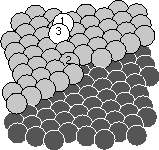
So, the picture above shows three of our surfaces. The big one was grown with the atoms gently set down onto the surface: no messy collisions, but the surface looks kind of bumpy. For this computer run, we could use just Kinetic Monte Carlo.
The two smaller ones look quite a bit flatter. They were grown using energetic,
high-velocity atoms. For these surfaces, each atom has a Molecular Dynamics
collision, leaving it and its neighbors splashed around on the surface.
Joachim's code then figures out what lattice site each atom belongs best to:
there are a few tricks here. Then he runs Kinetic Monte Carlo, allowing atoms
to hop occasionally and smooth out the surface, until its time for the next
collision.
Growing surfaces by spraying atoms on them is a big business! Your computer chips are metals and various dopants sprayed onto silicon: your disk drive heads are fancy `magnetic multilayers', sprayed on in just the right thicknesses to best read the bits on the disk. It's a great embarassment to the surface community that not only can't they grow surfaces in the shapes they want, they can't even grow them flat!
 Joachim figured out why the surfaces grew so flat, and it has to do with
the insertions and the pile-ups we discussed earlier. Joachim realized
that at the temperatures we grew at it is very hard for an atom to move
between layers except during one of the collisions. So, when one of the
collisions piles up an extra atom in an upper layer, it makes the surface
permanently rougher: that atom won't be able to move down to fill a hole
even during the enormous time between collisions. Insertions, on the other
hand, smooth out the surface: the atom flying in belonged to the third
layer, but ended up in the second layer, flattening things out.
Joachim figured out why the surfaces grew so flat, and it has to do with
the insertions and the pile-ups we discussed earlier. Joachim realized
that at the temperatures we grew at it is very hard for an atom to move
between layers except during one of the collisions. So, when one of the
collisions piles up an extra atom in an upper layer, it makes the surface
permanently rougher: that atom won't be able to move down to fill a hole
even during the enormous time between collisions. Insertions, on the other
hand, smooth out the surface: the atom flying in belonged to the third
layer, but ended up in the second layer, flattening things out.
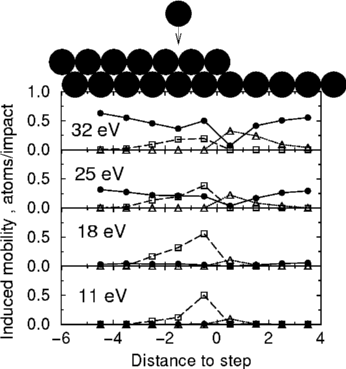
On the right above you see Joachim's graph, showing the good insertions
(white squares) and the bad pile-ups (white triangles). He started with
a straight edge like those pictured at the top, and plotted the number
of each depending on the distance from the step edge. For example,
the black atom hitting the step edge along the top of the graph is hitting
between -1 and -2 on the graph. (The black circles are adatom-vacancy pairs:
ignore them.) You can see at 18eV the good guys are winning a lot, and
at 25eV they are still doing well, but by 32 eV the bad guys begin to
win.
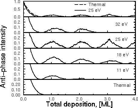 This picture works quite well. On the left you can see Joachim's graph showing
the layers going down one at a time. On this graph, large bumps mean smooth
layers. The bottom shows the surface grown with slow atoms, and gets rough
so quickly you don't see any bumps. The biggest bumps, and the smoothest
surfaces, happen at 18eV and 24eV: the surfaces where the good insertions
were most common and the bad pile-ups few and far between.
This picture works quite well. On the left you can see Joachim's graph showing
the layers going down one at a time. On this graph, large bumps mean smooth
layers. The bottom shows the surface grown with slow atoms, and gets rough
so quickly you don't see any bumps. The biggest bumps, and the smoothest
surfaces, happen at 18eV and 24eV: the surfaces where the good insertions
were most common and the bad pile-ups few and far between.
James P. Sethna, sethna@lassp.cornell.edu
 Statistical Mechanics: Entropy, Order Parameters, and Complexity,
now available at
Oxford University Press
(USA,
Europe).
Statistical Mechanics: Entropy, Order Parameters, and Complexity,
now available at
Oxford University Press
(USA,
Europe).
Statistical Mechanics: Entropy, Order Parameters, and Complexity,
now available at
Oxford University Press
(USA,
Europe).