Chaos!

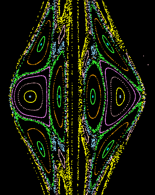
Jupiter here has a mass which is low enough (22000 Earth masses) so that the Earth's trajectory doesn't leave the solar system. This is a Poincaré section where we display a dot once each time the Earth passes Jupiter as both orbit the Sun. (That is, the Earth cuts through the Jupiter-Sun plane in the rotating coordinate system.) The dots represent the distance of the earth from the S-J center of mass, and the component of the velocity of the earth towards Jupiter. You can play with this by getting a copy of Jupiter (instructions below), and selecting the Preset for chaos.

Click the left mouse button to start a new trajectory! The Earth will be restarted at the parallel velocity and position that you input. (I got the idea of changing colors from John Guckenheimer's excellent program, dstool). Click and drag the right button to zoom; click without moving (or zoom out of the window) to back up to a broader view.

Notice the periodic orbits. If the Earth comes back to the same relative position each time it crosses the Jupiter-Sun axis, it'll always come out at the same point on the Poincaré section: an example is the second (pale blue) dot to the right of center. You get a dot when the Earth passes around the other side of the sun too: the dot on the far left of center is the same trajectory. If the Earth comes back to the same relative position every third time around, this leads to another periodic orbit (called a mode-locked state). The first dot to the right of center is such an orbit: the other two crossings between Jupiter and the Sun form the dots on the top and bottom right.

Notice the quasiperiodic orbits: the little bent circles scattered over the figure. They are KAM tori, representing non-chaotic ``quasiperiodic'' orbits. The torus, when it intersects the Poincaré section, cuts it in a closed curve. Each periodic orbit is surrounded by concentric tori. The six orange curves (three on each side) are obtained from starting the Earth in its standard initial condition:

Notice the chaotic orbits: the fuzzy regions filled up with dots. Trajectories in these regions are sensitively dependent on their initial conditions: at long times, one can't predict what will happen! You can test this by starting the program with initial conditions that differ a tiny amount, and watching the motion. Start in a chaotic region (by clicking the left mouse button at various points until the trajectory looks fuzzy).

Now, Configure the Initial Conditions, and change the Default Earth coordinates and velocities to agree with the current Earth X and Y coordinates and velocities. (The red numbers warn you that you need to hit enter after typing to enter the new values.) Hit Reset and Run, and make sure you've got the same trajectory you started with. (The dots should change color a few at a time: the new trajectory is writing over the old one.)

Now change one of the defaults (say, the Default Earth X-Coordinate) by a small amount (say 0.0001). Hit Reset and Run and watch the new dots. After a short while, they should stop overlapping! Try larger and smaller changes, and see how sensitive the motion is.

Now, try looking at the trajectories. Change the View to ``Earth's Trajectory''. Clear, Reset, and Run. You may want to view a larger region: clicking the right mouse button somewhere in the viewing area gives the default view, or click and drag to zoom in. Change the default by, say, 0.001, Reset, and Run. Watch the trajectories diverge!

Details of the Poincaré Section

In the rotating reference frame, there are four degrees of freedom (Rx, Ry, Vx, and Vy); conserving energy leaves us with three. This is special for two reasons. First, the Poincaré section of a three-dimensional system is two-dimensional: thus we can see the dynamics on the screen. Second, the KAM tori are two-dimensional surfaces: they have an "inside" only when embedded in three dimensions. In the planar, restricted three-body problem, a chaotic orbit surrounded by a KAM torus cannot escape! This happens also in particle accellerators (where the three dimensions are the x and y positions of the particle in the beam, and the angle along the circumference of the accellerator): otherwise the beam likely would leak out after the gizillions of orbits it makes. Stability is much more subtle when we allow Earth to influence Jupiter, or even when we allow motions in the third dimension: it is expected that all chaotic basins can get to one another, via a process called Arnold diffusion. Arnold diffusion is expected to be very slow, for small Jovian masses.

Three warnings. First, changing the mass (or any of a number of other things) will change the energy. If you don't clear the screen, you'll get the new orbits overlapping the old ones. Second, there are many places where there is no perpendicular velocity that conserves energy: the program will tell you VERBOTEN if you start in one of these areas (where the discriminant is negative). Third, the constant energy surface folds over when viewed from this perspective: if you click at negative R (the left half of the view) you'll see the back side of the energy manifold.

Short Questions

1. Observe the KAM tori (closed, smooth curves in the Poincaré section. Notice that they form concentric rings around periodic orbits. Describe the periodic orbits. What's the difference between the three you get by default, and the one in the upper right? (You can look at the animation or at Earth's orbit by shifting View. You'll want to click the right mouse button to remove the expanded scale.)
2. Find another set of KAM tori farther out, where the Earth is a moon of Jupiter. (You'll see both sides of the energy manifold: don't be confused by the overlapping tori: they're on different sheets.) It's separated from the solar orbits by a gap where the discriminant is negative (the VERBOTEN region). For this set of masses and energies, can the Earth swing around Jupiter? Find some allowed initial conditions at even larger radii. Can the Earth escape from the solar system? Why or why not?
3. Find the chaotic region (it's between the tori, and fills space). Are the trajectories dramatically different? Unzoom and look at the whole Poincaré section: what are the tails leading up and down in velocity? Does it look like the Earth can escape?
4. Find smaller KAM tori embedded in the chaotic region. You may want to change the dot size in "Configure". If you expand too much, you may get rounding errors: we'll need to explore the accuracy of the Runge Kutta, the number of digits in tcl_precision, and the number of digits written out by Jupiter.c to find out how to fix this.
5. Change the energy by increasing Jupiter's mass, or by changing the default initial velocity or position of the Earth (in "Configure"). Can you find a point where the Earth-Sun orbits first mingle with the Earth-Jupiter orbits? Where they both touch the orbits which leave the Solar System?

1. Basins: What does this conserved energy correspond to in the real (non-restricted) three-body problem? Does it guarantee stability, even in the absence of KAM tori? (Arnold tells us that, even for small Jovian masses, the KAM theorem breaks down when the Earth's orbit intersects that of Jupiter. Does the point where the solar and Jovian basins intersect mean anything special?
2. Arnold diffusion: For the non-planar problem, how long does Arnold diffusion take to connect two neighboring chaotic basins? How long to connect basins far away?

Jupiter:

• Description of the Three-Body Problem.
• Jupiter, Earth, and Sun
• Why hasn't the Earth left the Solar System?
• Invariant Tori
• Chaos!
• Lagrange Points
• Poincaré Section for the L5 Point
• Questions for Further Research

How to Get Jupiter

James P. Sethna, sethna@lassp.cornell.edu.

Statistical Mechanics: Entropy, Order Parameters, and Complexity, now available at Oxford University Press (USA, Europe).