The Restricted Three Body Problem
After Newton solved the problem of the orbit of a single planet around
the Sun, the natural next challenge was to find the solution for two
planets orbiting the Sun. Many of the best minds in mathematics and
physics worked on this problem in the last century.
Integrability
The first work went into finding an exact solution in analogy with the
two-body problem. It was quickly recognized that the key was to find
a sufficient number of conserved quantities. Energy, momentum, angular
momentum, and a weird vector provide enough information to solve the
two body problem. For problems where there are enough integrals,
the motion is quasiperiodic: roughly speaking, there are several
interdependent periodic motions, leading to a motion in phase space which
lies on a multi-dimensional
torus.
After a while, it was proven that there were not enough conserved quantities:
the three body problem is not ``integrable''.
Restrictions and ``Energy''
Gradually, the problem was simplified in order to explore the kernal of
the difficulty. The original eighteen-dimensional problem becomes
twelve when you move the center-of-mass coordinates. The planar
three-body problem, simplified by restricting the planets to a plane,
lies in eight dimensions. The restricted three-body problem
sets one mass to zero: imagine Earth as a dust particle, wandering around
Jupiter and the Sun which orbit one another. We study the circular,
planar, restricted three-body problem: the eccentricity of Jupiter's orbit
is set to zero.
The current state of our model is given by five numbers: the position
of Jupiter along it's orbit, and two velocities and positions for the
Earth. One of these can be removed by moving to a coordinate system
which rotates with Jupiter. Earth's angular momentum and energy are not
conserved, because Jupiter provides an external periodic force. However,
there is a conserved quantity
 which is output as the ``Energy'' in the program. Thus the motion of
the dust particle representing the Earth lies on a three-dimensional
surface of constant ``Energy'', in the rotating reference frame.
which is output as the ``Energy'' in the program. Thus the motion of
the dust particle representing the Earth lies on a three-dimensional
surface of constant ``Energy'', in the rotating reference frame.
Algorithm
We use variable time-step Runge Kutta to integrate the equations of motion,
using the Numerical Recipes routine odeint and rk4, suitably modified.
Runge-Kutta is not the ideal approach to simulating Hamiltonian systems:
even when it is quantitatively accurate, it is not qualitatively
accurate. In particular, what small errors are left will not conserve
energy (which will tend to drift up or down), and will violate Liouville's
theorem. We should be using a symplectic algorithm, for which
each time step is a canonical transformation. The classical Leapfrog
or Verlet algorithm for molecular dynamics is an example of a symplectic
algorithm: each time step is a canonical transformation, so it exactly
conserves an approximate energy (rather than approximately conserving
the real energy). Unfortunately, Verlet doesn't work with our periodically
forced systems, even in the rotating reference frame.
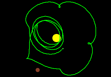
Poincaré Sections
Visualizing periodic trajectories is easy, but when they get
quasiperiodic or chaotic it's easier to use a Poincaré section.
That is, one defines a hyperplane in the phase space, and draws a dot
whenever the trajectory passes through the plane. This also
provides a mapping from the plane to itself (the Poincaré first-return
map), explaining why people use maps to understand dynamical systems
even when most practical systems are continuously evolving.
For our problem, I tried a lot of different maps. Taking a snapshot
once each Jovian year seemed natural, but leaves one with four coordinates
for the Earth: projecting the four dimensional space to two lost a lot
of information. The projection used in the program is where the Earth
lies directly between Jupiter and the Sun (the plane
rE x rJ = 0 for rE . rJ > 0).
If you select ``Poincare (rotating reference frame)'' under View,
the program will plot the distance from the earth along the axis
to Jupiter along the horizontal axis, and the velocity component
towards Jupiter along the vertical axis (the parallel components
of the distance and the velocity). The perpendicular component of the
position is of course zero; the perpendicular component of the velocity
is not shown.
If you click on the graphics screen while viewing the Poincaré
section, you'll start another trajectory with the appropriate parallel
positions and velocities. The program selects the perpendicular velocity
so that the ``Energy'' is conserved; if that's not possible, it writes
a note to the original window and plots nothing. Thus, you can view
a two-dimensional cross-section of the three-dimensional constant ``Energy''
surface.
Questions
- Who were the mathematicians and physicists who made serious
contributions to the theory of the three-body problem? In particular,
who proved that there were no further analytic integrals of the motion?
Can you provide Mosaic links to bios already on the Net for these?
- What is the ``weird vector'' which provides the last integrals
for the inverse-square two-body problem? Find out how it's related
to the mapping from the inverse-square 3-D problem to the four-dimensional
harmonic oscillator. How does it relate to the Laplace vector?
- Show that the ``Energy'' defined above is conserved. (What's its
real name?) If we make
the mass of the earth finite, the real energy and angular momentum
are conserved. How do these turn into ``Energy'' in the limit where
the earth's mass goes to zero? What happens to the other conserved
quantities?
- Figure out what symplectic means.
Implement a symplectic algorithm, and check whether it runs faster
than Runge Kutta. See, e.g.
Olver, P. J., "App. of Lie Groups to Diff Eqn's" QA372.052, 1993 or
Sanz-Serna, J. M., "Numerical Hamiltonian Problems" QA614.83.S26x.1994
in the Math library.
Jupiter:
How to Get Jupiter
Jupiter is available
for Windows 95, Windows NT, Macintosh, and several Unix platforms
(the IBM RS6000, Sun Sparc, Dec Alpha (courtesy Kamal Bhattacharya),
Linux, and the PowerPC running AIX4.1).
The files are available without charge by anonymous FTP
(ftp.lassp.cornell.edu) or
via
the World Wide Web.
Last modified: May 19, 1996
James P. Sethna,
sethna@lassp.cornell.edu.
 Statistical Mechanics: Entropy, Order Parameters, and Complexity,
now available at
Oxford University Press
(USA,
Europe).
Statistical Mechanics: Entropy, Order Parameters, and Complexity,
now available at
Oxford University Press
(USA,
Europe).

