H3: Double Slit Diffraction

Now, we turn to the diffraction through double slits, where the width of the slits a is not tiny compared to the distance d between their centers. Load the preset DblDiff. Notice that we now have two slits of width a=2 m separated by d=6 m.

(H3a) Connection with two point slits.

Measure the position of the first minimum. Compare to the position of the first minimum of two thin slits. You can calculate this if you like, but we'll do the comparison graphically. Change Your Name to your name, and use copy graph to store the double-slit diffraction pattern. Change to a=0, and use steal data to combine the two graphs. Notice that the double-slit diffraction pattern has the same minima as that of the thin-slit diffraction pattern. You may want to use configure on the graph window to change colors and names for the two curves. You can use save postscript to create a PostScript file for the plot, and print it out. Include this plot in your write-up. (Plots with your correct name on them may be required by your TA. Under some circumstances, your TA may announce that they will accept careful sketches - but typically only from those who turn the labs in on time!)

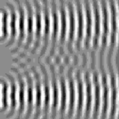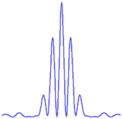
Can we understand this? Think of the total wave impinging on the screen from the bottom slit. It has an amplitude which is a complicated formula, but the form is just a sine wave with a phase. The total wave impinging on the screen from the top slit is a sine wave with about the same amplitude, but a phase that is different because the top slit is a fraction of a wavelength different in distance. This difference in distance is just the same as it would be for two thin slits - so the condition for destructive interference is the same!

(H3b) Comparison with the single slit pattern.

Reset a=2 (or preset again to DblDiff). Notice that the peaks get smaller, one peak seems to be almost missing, and then the peaks grow larger again.

Change to one slit. The fast wiggles disappear, but the overall shape looks the same! We can compare these two plots graphically in the same way as we did for part H3a. Change back to two slits, and use copy graph to store the pattern. (Make sure your name is on the plot.) Change to one slit. Notice that the peak is at a different height: four times as much intensity hits Y=0 when two slits are open. Explain in your write-up why this is happens. (Hint: amplitudes add; we're plotting the intensity.) Four times the intensity at the center, from twice as many openings, is OK: after all, in the dips you get zero times the intensity when you double the number of slits!

Before steal data, we have to make the peaks the same height. Using configure... on the huygens window, change the Wave Amplitude/Area to make the peak of the single-slit pattern the same height as that of the double-slit pattern you've stored in graph1. (Don't do this by trial and error! How much larger amplitude do you need to multiply the intensity by four?) Now, use steal data, print the plot, and include it (or a careful sketch, if it's cleared first with your TA) in your write-up.

We can understand this by using the same argument we did in H3a. The amplitude for the double slit is the superposition of two single-slit amplitudes, with a phase shift between them. Where the interference between these two waves is constructive, the amplitude is exactly twice that of the old single-slit pattern (the intensity is up by a factor of four). Anywhere else, the amplitude is less! This means that four times the single-slit pattern gives an upper envelope to the double-slit diffraction pattern, just as we observe.

Links Back

Statistical Mechanics: Entropy, Order Parameters, and Complexity, now available at Oxford University Press (USA, Europe).