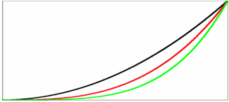
Sloppiness comes from parameters which affect the predictions in similar ways. Here the monomials x3, x4, and x5 all are flat near zero, and increase smoothly near one. We can trade the coefficient a4 for a suitable combination of a3 and a5, and get almost exactly the same final function.

Fitting Polynomials: Where is sloppiness from?

Multiparameter models are usually sloppy - their parameters can vary over huge ranges without changing the fits to data very much. Where does this sloppiness come from? We provide three answers to this question, all really the same answer in disguise.

Consider the standard problem of fitting polynomials to data. Our model is a sum of monomials xⁿ, with coefficients a_n:

1. Sloppiness comes from having groups of parameters whose effects can be traded for one another.

Indeed, if we are fitting a continuous function in the range between zero and one, we can explicitly calculate the Hessian matrix whose range of eigenvalues we use to decide whether the system is sloppy. This Hessian is the Hilbert matrix:

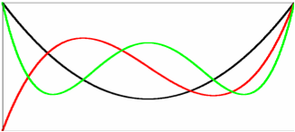
Changing the parameters can remove the sloppiness. When fitting polynomials to data, one is told to vary not the monomial coefficients an, but the coefficients bn of a suitable class of orthogonal polynomials: here the shifted Legendre polynomials Ln. Here are plotted L3, L4, and L5. By design, these polynomials can't be traded for one another. The same polynomial fit to the same data, expressed in terms of new variables bn, is not sloppy.

Those readers who actually have fit polynomials to data will remember, though, that one doesn't usually calculate the monomial coefficients a_n. Instead, one fits to a sum of orthogonal polynomials

2. Sloppiness comes from the way we choose the variables in our theory.

Notice that in the case of fitting polynomials, we often don't think that the monomial coefficients are very important: the b variables are almost as natural as the a variables. But in a biological model or an engineering system, the variables we use are usually natural and sensible, and using strange combinations of variables just to avoid sloppiness will usually not make scientific sense.

Skewness. The change of variables from the bare parameters (monomial coefficients an) to parameters natural to the model (coefficients of the orthogonal polynomials bn is not a rotation in parameter space. It is more of a tortured, skewed stretching. The red arrows represent the change in natural coordinates when different bare coordinates are varied. Notice that one can get to nearly the same final behavior (tip of the skewed cube) by going along any of the three bare coordinates (they all affect the predictions in similar ways). Notice also that the volume of the skewed cube is small; it is proportional to the determinant of the mapping from bare to skewed coordinates.

Why did changing from the monomial coefficients a_n to the orthogonal polynomial coefficients b_n make such a big difference? Unlike many familiar transformations, this change is not just a rotation (in six-dimensional function space); it is instead a very skewed, shearing kind of transformation (figure at left). The meaning of "perpendicular" in parameter space is subtle: most scientifically natural choices for parameters are sloppy for this reason.
3. Sloppiness comes a severe skewness between the scientifically natural "bare" parameters and the parameters naturally governing the model behavior.

Can we understand the key properties of sloppy models mathematically? See Why sloppiness? The Sloppy Universality Class

References

• "Sloppy model universality class and the Vandermonde matrix", Joshua J. Waterfall, Fergal P. Casey, Ryan N. Gutenkunst, Kevin S. Brown, Christopher R. Myers, Piet W. Brouwer, Veit Elser, and James P. Sethna, Phys. Rev. Letters 97, 150601 (2006), pdf.
• Other papers on sloppy models

More on sloppiness:

• Sloppy Models
  • A sloppy systems biology model
  • What is Sloppiness?
  • What are Sloppy Models?
  • Fitting Exponentials: Prediction without parameters
  • Fitting Polynomials: Where is sloppiness from?
  • Why sloppiness? The Sloppy Universality Class
  • Differential Geometry and Sloppy Models (Transtrum)
    • The Model Manifold and Hyperribbons (Transtrum)
    • Sloppy Curvature (Transtrum)
  • Why is science possible? Sloppy models in Physics.
    • Jessie Silverberg's Huffington Post article and Katheryn McGill's vlog Interview from The Physics Factor.
    • Unedited workshop interview by Steven Reiner, Stony Brook School of Journalism; Mobile version.
• Sloppy model applications
  • Do parameters matter? Fits versus measurements.
  • Experimental design in sloppy systems
  • Robustness and sloppiness
    • Parameter robustness and sloppiness
    • Environmental robustness and sloppiness: Circadian rhythms
    • Evolvability, robustness, and sloppiness
  • Estimating systematic errors for interatomic potentials and for density functional theory.
  • Learning digits with InPCA

James P. Sethna, sethna@lassp.cornell.edu; This work supported by the Division of Materials Research of the U.S. National Science Foundation, through grant DMR-070167.

Statistical Mechanics: Entropy, Order Parameters, and Complexity, now available at Oxford University Press (USA, Europe).