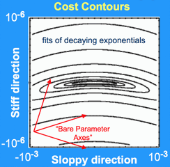
Banana-shaped sloppy valley. Cost contours for a sloppy model of exponential decay. The horizontal and vertical axes were chosen in the sloppiest and (second) stiffest directions. Notice that the horizontal axis is squashed by a factor of a thousand - our figure should really be stretched horizontally to roughly half the size of a sports arena. The aspect ratio is roughly that of a human hair.

What are Sloppy Models?

James Sethna > Sloppy Models > What are Sloppy Models? We claim that many if not most models with several fitting parameters (say, more than five) are sloppy. Sloppy models are called 'poorly constrained' and 'ill-conditioned' because it is difficult to use experimental data to figure out what their parameters are. Suppose the data y_i=y(t_i) is being fit by a model y(θ,t) with parameters θ=&theta₁, &theta₂, ... &theta₁₇, ... We can measure the quality of the fit to the data by defining a cost C, the sum of the squares of the differences between theory and experiment (sometimes called χ²):

The figure at left shows a contour plot of this cost for one of our sloppy models (fitting exponentials), zoomed in near the best fit at the center. Crossing contours corresponds to increases in cost; the system behavior predicted by the model no longer agrees as well with the data. The horizontal and vertical axes move in certain carefully chosen stiff and sloppy directions in parameter space (along eigenparameters that we describe below). Notice first that the behavior changes much less as we move the parameters in the sloppy, side-to-side direction, than if we change them along the vertical stiff direction. Notice second that we have squashed the plot by a factor of a thousand; the sloppy direction is really enormously less constrained than the stiff direction.

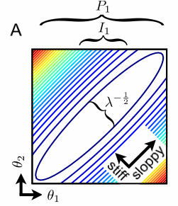
Stiff and sloppy directions in parameter space. Moving up and right in parameter space changes the system behavior very little, so few contours are crossed - a sloppy direction. Moving up and left in parameter space changes the system behavior rapidly - a stiff direction. The length of the axes of the ellipses are given by the square roots of the eigenvalues. For sloppy multiparameter models, there is an enormous range of eigenvalues - only a few eigenparameters are well determined by the data.

Eigenvalues and eigenparameters

The banana-shaped contour plot above is a two-dimensional cross-section of the cost in a large-dimensional parameter space. How can we describe the behavior as we change the parameters in a general direction?

Near enough to the best fit, we almost always will find that the cost contour surfaces form ellipsoids - stretched long along sloppy directions, and pinched in along the stiff directions. These ellipsoids can be described by the eigenvalues and eigenvectors of the Hessian H_αβ = ∂²C/∂θ_α∂θ_β of the cost near the best fit. The eigenvectors point along the different axes of the ellipse; we call these parameter combinations eigenparameters, as opposed to the bare parameters that we originally chose to write our model in terms of. The eigenvalues λ_n are the squares of the lengths of the ellipsoids along the different eigenparameters.

We can see from the schematic figure at left that the behavior does depend sensitively on the value of the bare parameter θ₁; we cross contours as we move horizontally almost as rapidly as if we moved along the stiff eigenparameter up and to the left. But the error bar P₁ for bare parameter θ₁ is big because of the sloppy direction. One can't use the system behavior to determine θ₁ because it can be exchanged for θ₂ with little change in cost, moving along the sloppy direction.

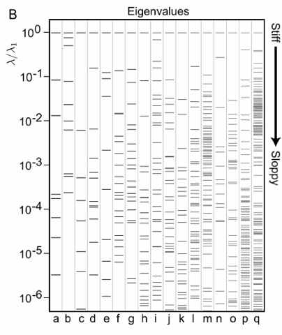
Sloppy systems biology eigenvalue spectra. The eigenvalues of all of these models are spread rather uniformly over more than six decades (corresponding to an aspect ratio of over a thousand between stiffest and sloppiest directions). The systems analyzed here cover everything from fruit fly embryo formation, to the metabolism of nucleotides for DNA, to biological clocks, to hormonal signal transduction.

Sloppiness in systems biology, math, and physics.

We first encountered sloppiness in a systems biology model of the response of a certain cell to hormones. The eigenvalues for that model are shown in the figure at right in column (i). We were struck by the fact that the 48 eigenvalues in that model were roughly equally spread over six decades. (A few eigenvalues near zero might be something weird with the model, but such nicely spread-out eigenvalues seemed like it might be there for a reason.) Ryan Gutenkunst then took sixteen other systems biology models from the literature, covering everything from fruit fly embryo formation, to the metabolism of nucleotides for DNA, to biological clocks. All of these models had many parameters, and when we studied the change in experimental behavior as we varied the parameters we found that they too shared the same sloppy features (right, a-q). That is, they all had an enormous range of eigenvalues, with a few stiff combinations of parameters that were well constrained by the data and many sloppy combinations, which can vary by vast amounts without significant change in the system behavior.

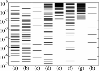
Sloppy (and non-sloppy) eigenvalues from many fields. (a) our systems biology model; (b) quantum Monte Carlo variational wavefunction; (c) radioactive decay for a mixture of twelve common nuclides; (d) fit of 48 exponential decays; (e) random 48x48 matrix (GOE, not sloppy); (f) product of five 48x48 random matrices (not sloppy, but exponentially spread), (g) multiple linear regression fit of a plane to data in 48 dimensions (not sloppy), and (h) a polynomial fit to data (sloppy).

Is sloppiness special to biological systems? Apparently not! We've found sloppiness in multiparameter models spanning many fields, from models of insect flight, to interatomic potentials, to accelerator design - every multiparameter model that we have studied so far appears to be sloppy. At left you can see a few examples. Quantum Monte Carlo, for example, is our most precise tool for solving for the energies and quantum behavior of atoms and small molecules; Cyrus Umrigar's wonderfully accurate variational wave-functions underlying this method, however, are remarkably sloppy (column b). Precise predictions can be made from sloppy models. In mathematics, fitting sums of exponential decays to radioactivity data (columns c and d) can give excellent fits with decay constants that are wildly different from the true ones - a classic example of an ill-posed fitting problem. Finally, fitting polynomials to data is sloppy, at least insofar as one is interested in the coefficients of the polynomials (column h).

To gain more intuition about how predictions are possible without good parameters, see Fitting Exponentials: Prediction without parameters.

References

• "Universally Sloppy Parameter Sensitivities in Systems Biology", Ryan N. Gutenkunst, Joshua J. Waterfall, Fergal P. Casey, Kevin S. Brown, Christopher R. Myers, James P. Sethna, PLoS Comput Biol 3(10) e189 (2007). (PLoS, doi:10.1371/journal.pcbi.0030189), pdf). [Reviewed in NewsBytes of Biomedical Computation Review (Winter 07/08).]
• Other papers on sloppy models

More on sloppiness:

• Sloppy Models
  • A sloppy systems biology model
  • What is Sloppiness?
  • What are Sloppy Models?
  • Fitting Exponentials: Prediction without parameters
  • Fitting Polynomials: Where is sloppiness from?
  • Why sloppiness? The Sloppy Universality Class
  • Differential Geometry and Sloppy Models (Transtrum)
    • The Model Manifold and Hyperribbons (Transtrum)
    • Sloppy Curvature (Transtrum)
  • Why is science possible? Sloppy models in Physics.
    • Jessie Silverberg's Huffington Post article and Katheryn McGill's vlog Interview from The Physics Factor.
    • Unedited workshop interview by Steven Reiner, Stony Brook School of Journalism; Mobile version.
• Sloppy model applications
  • Do parameters matter? Fits versus measurements.
  • Experimental design in sloppy systems
  • Robustness and sloppiness
    • Parameter robustness and sloppiness
    • Environmental robustness and sloppiness: Circadian rhythms
    • Evolvability, robustness, and sloppiness
  • Estimating systematic errors for interatomic potentials and for density functional theory.
  • Learning digits with InPCA

James P. Sethna, sethna@lassp.cornell.edu; This work supported by the Division of Materials Research of the U.S. National Science Foundation, through grant DMR-070167.

Statistical Mechanics: Entropy, Order Parameters, and Complexity, now available at Oxford University Press (USA, Europe).